All published articles of this journal are available on ScienceDirect.

Rapid Pre-construction Forecasting of Schedule Overruns: A Machine Learning Regression Approach

Abstract
Introduction/Objective
This study developed and validated a parsimonious machine-learning regression model that estimates schedule overruns for building construction projects prior to project start.
Methods
Using a dataset of 60 completed building projects in Lebanon, each with 11 pre-project predictors, an XGBoost regression model was trained and tested on an independent dataset, with repeated cross-validation and hyperparameter tuning.
Results
Averaged over repeated randomized train/test partitions, the trained and tuned model achieved an R2 = 79.6% (adjusted R2 = 74.3%), a mean absolute error of 4.36 ± 0.48 percentage points (95% CI: 3.42–5.30), and a median coverage near the nominal 90% for empirical prediction intervals.
Discussion
The regression-based approach extends existing delay-risk assessment by estimating delay magnitude rather than only the risk class, while factor-importance analysis identified owner/client performance, legal/permit issues, design quality, and project manager experience as the major drivers of delay.
Conclusion
The model provides a practical decision-support tool for project managers to estimate the expected magnitude of delay and its uncertainty before construction initiation, requiring only eleven readily obtainable pre-project inputs.
1. INTRODUCTION
The construction industry is one of the largest industries globally. It represents close to 9% of the GDP in many countries [1]. However, it is plagued by challenges that frequently lead to claims and disputes among the involved parties [2]. Improving construction project performance across the essential three pillars of cost, schedule, and quality remains a significant challenge to contractors [3]. Successful construction projects are defined by their completion within budget, on schedule, and in accordance with specified quality [4, 5]. Contractors try to increase profits and market share by identifying critical success factors and evaluating their impacts prior to project start [6]. Project delays represent one of the most significant challenges facing the global construction sector, with only 25% of projects reportedly finishing within 10% of their contract-planned completion dates [6-8]. Delays can arise from reasons related to contractors, owners, designers, and external factors [6]. Although technological advancements have been made, project delays remain a persistent issue in the industry [9]. The implications of these delays extend beyond just schedule overruns and often lead to increased costs, loss of productivity, heightened disputes, and potential contract termination [10].
Traditional scheduling methods for determining project duration, such as the Critical Path Method (CPM) and Program Evaluation Review Technique (PERT), are commonly utilized in project management software [11, 12]. However, due to their inherent limitations and the complex nature of construction projects, overruns persist, prompting contractors to employ activity crashing strategies [13]. Recent research underscores the need for innovative technological approaches, particularly in forecasting project durations [14]. Notably, there is significantly less scholarly focus on project duration issues compared to cost estimation [15]. The complexities inherent in construction projects, comprising numerous interconnected tasks, often complicate the identification of relationships among these tasks [11]. Machine learning presents a promising solution, demonstrating capabilities in analyzing extensive datasets and uncovering intricate relationships between variables [16]. Consequently, existing approaches either require relatively detailed project information or provide limited capability for directly estimating the magnitude of schedule overruns using information readily available before construction begins.
Despite existing research on construction schedule delays, a gap remains for practical pre-project models that directly estimate the magnitude of schedule overruns using a compact set of readily obtainable inputs. To address this gap, this study develops a compact, interpretable regression model that predicts delay magnitude rather than class membership. By requiring only readily obtainable pre-project information and providing both an estimated delay magnitude and its uncertainty, the proposed approach reduces the need for detailed activity-level information while providing actionable information for early schedule-risk assessment. After synthesizing the literature on delay drivers, 11 readily obtainable pre-project predictors were selected and used to train an XGBoost regressor on 60 building projects. XGBoost was selected as the modeling framework because of its ability to represent nonlinear relationships and interactions in small tabular datasets while accommodating heterogeneous predictor types. The present study evaluates the performance and practical utility of this selected XGBoost approach; it was not designed as a comparative benchmark of alternative regression algorithms [17]. The study demonstrates that a small feature set can yield accurate, probabilistically calibrated delay estimates and identify dominant risk drivers. Contributions include (1) a regression-based forecasting tool for pre-construction delay magnitude, (2) an empirical assessment of a compact predictor set suitable for practitioner use, and (3) an interpretable output package (point estimate, prediction interval, ranked factors) to support early mitigation decisions.
1.1. Literature Review
Estimating the duration of a construction project is quite complex due to the existence of multiple interdependent activities, interdependent resources required, and the variability in crew productivity [18]. Various methods have been developed for this purpose, with differing levels of accuracy and complexity. The Critical Path Method (CPM), which is used by approximately 89% of U.S. contractors due to its simplicity, assumes deterministic values for activity durations, potentially compromising accuracy [19]. To account for potential delays, planners often add a “buffer” to the estimated duration, which can be estimated through comparison with similar past projects [13]. Limitations of CPM also include its failure to recognize shifting critical paths, which are typically managed by applying buffers that may not sufficiently reflect project-specific variables [11]. Some contractors calculate the buffer using a thorough risk analysis. This method results in much better accuracy, but it comes at the cost of a detailed analysis [19]. Only 33% of construction companies conduct such detailed analysis because of the skill and time needed to achieve results [12].
The Program Evaluation and Review Technique (PERT) enhances the CPM approach by incorporating three estimates for activity duration: optimistic, realistic, and pessimistic. This probabilistic framework allows for the calculation of the expected project duration and the likelihood of on-time completion. However, the complexity of gathering actual historical activity durations can deter project managers from using PERT, especially in large projects involving numerous activities [11, 19, 20]. The Probabilistic Network Evaluation Technique (PNET) improves upon PERT by accommodating the potential for any activity to impact the critical path, yet demands more extensive data input. Given the complexity of estimating durations for large construction projects with hundreds or thousands of activities, reliance on computer-based scheduling tools has become essential. Widely used software such as MS Project and Primavera P6 facilitates this process, with studies indicating that managers outside construction often prefer MS Project for its user-friendliness, while construction professionals favor Primavera P6 for its ability to manage complex projects [12, 14].
Schedule delays in building construction can result from a combination of factors: technical, contractual, managerial, and external factors. The most common factors reported in international studies include poor project management and supervision, inadequate planning and scheduling, design deficiencies and change orders, late delivery of materials, subcontractor performance issues, and owner-related problems such as unclear requirements or slow decisions [6, 21, 22]. Other factors like probabilistic and resource uncertainties, unforeseen site conditions, and inadequate risk allocation further increase schedule overruns [11, 13]. Institutional limitations and macroeconomic instability influence the causes of project delays. In developing countries, client and financing issues, administrative and permitting constraints, and supply-chain disruptions are frequently reported. Consequently, local context influences the relative importance of delay factors [6, 21].
Artificial Intelligence (AI) has found growing applications in construction [23]. Machine Learning (ML), a subset of AI, enables systems to learn and adapt over time. Despite the construction sector being one of the least digitalized industries, recent applications of AI and ML, such as estimating materials for construction [24], assessing labor safety risks [25], and predicting the performance of construction crews [26], demonstrate their growing potential. XGBoost, an ML algorithm [27], has been shown to be efficient and accurate in data analysis, especially in regression tasks [16]. Boosting methods improve predictive performance by combining successive decision trees to reduce model errors. XGBoost accommodates missing values and includes regularization mechanisms that help control overfitting. These capabilities support its application to heterogeneous construction data [28]. It uses K-fold cross-validation to enhance the accuracy of ML models by partitioning the dataset into K subsets, allowing for effective testing and training processes that utilize more data [16].
Many AI-based approaches to project scheduling classify projects by delay risk rather than estimate the magnitude of schedule overruns. Existing machine learning approaches differ in their methods and input requirements. For instance, fuzzy logic was used to adjust durations [18], and neural networks were used to successfully sort delay risks [29]. However, their data and input requirements may limit their use before construction begins. This study develops a compact model that uses readily obtainable pre-project inputs to provide construction teams with an estimate of delay magnitude.
1.2. Research Methodology
Extant reviews and meta-analyses were synthesized to compile a candidate list of delay factors commonly reported in the literature [6, 30]. The syntheses highlight recurring causes of delays such as client/owner issues, permitting/legal obstacles, design deficiencies, material and subcontractor delays, and project management shortcomings, which informed our selection of pre-project predictors [29, 31, 32].
Previous studies show that project context varies substantially, particularly across developing countries. Accordingly, the focus was on risk factors consistently reported across regions and project types [33]. Keeping the predictor set small and compact was a deliberate choice. Recent literature supports practical, data-driven tools that use information available before project commencement [34, 35]. Eleven primary delay factors were selected and expressed as measurable variables linked to specific survey questions (see Table 1). The confidential questionnaire was then distributed to several construction firms in Lebanon. Companies could submit data for one or more projects, resulting in a dataset of 60 completed building projects in Lebanon. The study was restricted to building projects because schedule delays depend on project type. Application to infrastructure projects or other regions would require additional data and model retraining. For variables representing supplier/subcontractor reliability, stakeholder performance, and external risks, the collected values were intended to characterize information available at project commencement, including historical performance/reliability and anticipated risks, rather than adverse events that subsequently occurred during project execution. For example, supplier and subcontractor variables represented their historical frequency of delayed performance, while municipality-related risk reflected the likelihood of problems expected at project commencement.
| Cause of Delay | Quantifiable Factor | Questionnaire Question | Unit |
|---|---|---|---|
| Inadequate contractor experience | Years of experience of project manager | How many years of experience did the project manager have upon starting the project? | Years |
| Poor site management and supervision | |||
| Change orders and slow decision making | Quality of design documents Owner’s desires were clear and concise |
How would you rate the owner’s performance during the project? | Poor – Average – Good |
| Late delivery of material | Percentage of late deliveries to site | On average, how often are suppliers late in their site deliveries? | Percentage |
| Unreliable subcontractors | Percentage of subcontractor tasks that face delay | On average, what percentage of subcontractor tasks experience delays? | Percentage |
| Percentage of the project that was subcontracted | What percentage of the project was subcontracted? | ||
| Delay in performing inspection and testing | Consultant performance | How would you rate the consultant performance? | Poor – Good |
| External factors: political issues, paperwork issues and weather-caused delays | Were there issues with municipality and neighbors that caused construction delays? | Did the project face legal issues and problems with the municipality and/or neighbors? | Yes / No |
Extreme Gradient Boosting (XGBoost) was chosen for regression modeling due to its strong empirical performance, ability to combine many shallow decision trees into a robust ensemble, and effective handling of heterogeneous feature types and missing values.
XGBoost generates predictions by summing the contributions (leaf values) from each tree in the ensemble for a given observation. Each successive tree is trained to correct the residual errors of the preceding ensemble, producing a boosted model comprised of many trees. For prediction, a new observation is propagated through each tree, and the estimated delay is obtained as the sum of the contributions from the terminal leaves reached across the ensemble.
The dataset was partitioned into training (75%) and testing (25%) sets. Model selection and hyperparameter tuning were performed using 10-fold cross-validation on the training set. Final model performance was evaluated on the held-out testing set. To reduce sampling variability, the three-stage process (split → cross-validation training → test evaluation) was repeated 1000 times; reported metrics are the means across repetitions. These repetitions were used to assess the sensitivity and stability of model performance across different train–test partitions of the 60 available projects; they do not represent additional independent observations or external validation.
The data were separated into a model-development set and a final held-out test set before model training. Hyperparameter tuning was conducted exclusively within the model-development set using [cross-validation/ resampling/internal validation split]. The final test set was not used for hyperparameter selection, model comparison, feature selection, or any other modeling decision. After the hyperparameters and final model specification had been fixed, the model was evaluated once on the held-out test set using MAE and R2.
Categorical and ordinal survey responses were numerically encoded for modeling. Examples: design quality (0 = poor, 1 = average, 2 = good), consultant performance (0 = poor, 1 = good), project complexity (0–2 scale), and legal/municipality issues (binary 0/1). Continuous variables (e.g., estimated duration, percentages) were retained in their native units.
1.3. Hyperparameter Tuning
Hyperparameter tuning was undertaken to maximize model generalization while avoiding overfitting [36]. Hyperparameter optimization was conducted in two stages. First, a coarse grid evaluated combinations of the principal XGBoost hyperparameters, including tree depth, learning rate, number of estimators, subsampling, column subsampling, and regularization parameters. This stage allowed the joint performance of representative hyperparameter combinations to be assessed. Second, one-dimensional sweeps were conducted around the best-performing region to refine selected parameters. This approach does not exhaustively characterize all higher-order interactions among hyperparameters, but it provides a computationally practical refinement strategy while retaining joint evaluation of the main parameter combinations in the initial stage. Model performance during tuning was assessed by 10-fold cross-validation on the training set and by mean MAE and R2 across repeated randomized train/test partitions. This approach balanced exploration of the search space with computational tractability, reducing the risk of selecting values that overfit a single split.
Optimization robustness was assessed by repeating the complete train/test partitioning, cross-validation, and test evaluation procedure 1000 times with different randomized partitions. For each repetition, the tuning procedure was conducted using only the training portion, and performance was recorded on the corresponding held-out test portion. The resulting distributions of MAE and R2 were summarized using their means, standard deviations, and 95% confidence intervals.
1.3.1. Maximum Tree Depth
The maximum tree depth (max_depth) controls the maximum number of splits permitted in each tree and therefore governs the per-tree complexity. Values in the range 1–6 were tested. Among the candidate depths evaluated, a maximum depth of 2 produced the best validation performance. It improved cross-validated R2 relative to depth = 1 while avoiding the overfitting observed for depth ≥ 3, where validation performance and Mean Absolute Error (MAE) deteriorated. Consequently, max_depth was fixed at 2 to favor many small trees that together capture interactions without producing excessively complex individual trees.
1.3.2. Number of Trees
The number of boosting iterations (n_estimators) determines how many trees are included in the ensemble. Values from 50 to 100 were evaluated in increments of 10. Among the candidate values evaluated, 70 trees produced the best validation performance; increasing the number of trees beyond this point produced negligible improvement and, in some folds, slightly increased variance. Based on this behavior and computational considerations, n_estimators was set to 70.
1.3.3. Learning Rate
The learning rate (eta) scales the contribution of each added tree and mediates the trade-off between the number of trees and the stability of learning. A fine sweep around common defaults (0.08–0.12) was performed. Performance plateaued at a learning rate of 0.1: lower values required substantially more trees for marginal gain, while higher values increased sensitivity to noise. Thus, eta = 0.1 was selected to balance convergence speed and generalization.
1.3.4. Subsample
Row subsampling (subsample) and column subsampling per tree (colsample_bytree) introduce stochasticity that reduces overfitting and the influence of outliers. Subsample values between 0.5 and 1.0 were tested; a subsample of 0.7 produced the best cross-validated R2 and lowest MAE, with smaller values tending toward underfitting and larger values reducing regularization. For column sampling, values within the same range were evaluated, and colsample_bytree ≈ 0.8 delivered the best validation metrics; lower values reduced feature coverage, while higher values slightly increased overfitting. Accordingly, subsample and colsample_bytree were fixed at 0.7 and 0.8, respectively.
1.3.5. L1/alpha Regularization (Lasso regularization)
Regularization was used to penalize overly complex models and reduce reliance on weak predictors. An L1 (alpha) regularization sweep over 0.01–0.2 indicated that a modest L1 penalty of 0.1 yielded a small but consistent improvement in MAE and encouraged sparsity in leaf weights without degrading fit.
Parameters primarily intended to control complexity in deep trees, gamma (minimum loss reduction required for a further split) and min_child_weight (minimum sum of instance weight needed in a child) were found to have negligible influence given the shallow max_depth = 2 and were therefore left at their default values. The final hyperparameter values are shown in Table 2.
| Hyperparameter | Final Value |
|---|---|
| max_depth | 2 |
| n_estimators | 70 |
| learning_rate (eta) | 0.10 |
| subsample (row subsample) | 0.7 |
| colsample_bytree (feature subsample) | 0.8 |
| alpha (L1 regularization) | 0.10 |
| min_child_weight | 1 (default) |
| gamma | 0 (default) |
1.4. Dataset Summary and Descriptive Statistics
The dataset comprised 60 building projects. Key descriptive statistics and variable ranges are summarized in Table 3 (e.g., estimated duration, actual duration, delay days and percentage, supplier/subcontractor delay percentages, project manager experience, percentage subcontracted, days saved by crashing). Encoded categorical distributions are shown in Fig. (1) (design quality, consultant performance, project complexity, legal issues, and client performance).
| Factor | Minimum Value | Maximum Value | Average Value |
|---|---|---|---|
| Estimated duration (days) | 60 | 1464 | 443 |
| Actual duration (days) | 75 | 1584 | 549 |
| Delay (days) | 0 | 360 | 106 |
| Late supplier deliveries (%) | 20 | 30 | 22 |
| Tasks where subcontractor is delayed (%) | 15 | 35 | 29 |
| Project manager years of experience | 5 | 35 | 18 |
| Subcontracted part of the project (%) | 0 | 100 | 38 |
| Days saved by crashing | 0 | 90 | 31 |
| Consultant performance | Poor | Good | - |
| Project complexity | Familiar | Highly complex | - |
| Issues faced with municipality and neighbors | No | Yes | - |
| Owner’s performance | Poor | Good | - |
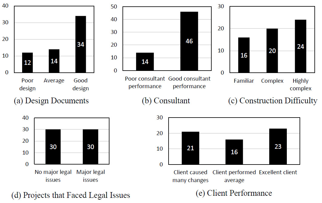
Encoded categorical distributions.
The model was implemented in Python. The deployed tool prompts the user for 11 inputs corresponding to the selected predictors, as shown in Fig. (2). Outputs comprise: (1) a point estimate of project delay (percentage), (2) a 90% prediction interval computed from the empirical error distribution, and (3) the three features contributing most to the predicted delay for the given input. The 90% empirical prediction interval was constructed from the empirical distribution of prediction errors, defined as
 . The 5th and 95th percentiles of this error distribution were obtained and added to the point prediction, such that the interval for a prediction
 was
 . The resulting interval therefore represents an empirical estimate of predictive uncertainty rather than a parametric confidence interval.
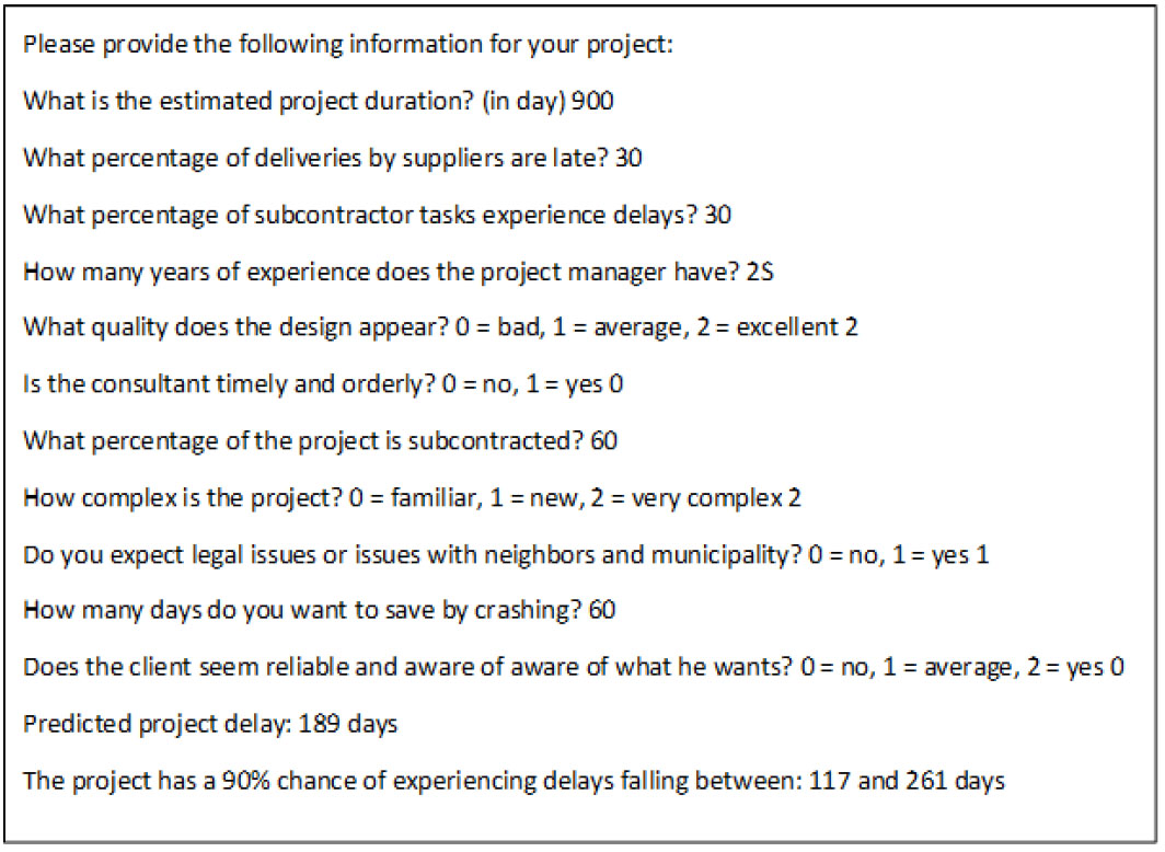
Sample inputs and outputs of the model.
1.5. Case Illustration
To demonstrate the model’s mechanics, a representative test observation was processed by the trained XGBoost ensemble composed of 70 trees. Each tree returned a leaf value for the observation; the predicted delay percentage is the sum of the leaf contributions across all trees. In the illustrative case, the ensemble predicted a 25% delay, compared with the observed 19%, demonstrating how the ensemble aggregates many small contributions to produce the final estimate.
A representative test case is presented to illustrate XGBoost prediction mechanics. The model was trained on the training set, and a single observation from the held-out test set was passed through the trained ensemble. The ensemble comprised 70 trees; Fig. (3) displays four example trees. Rather than relying on a single decision tree, the XGBoost predictor aggregates the contributions of all trees: each tree returns a leaf value for the observation, and the final predicted delay equals the sum of these leaf values. In this implementation, each tree considered three of the eleven available features, and more influential features were selected more frequently during tree construction. This ensemble approach produces more stable and accurate point estimates than a single decision tree.
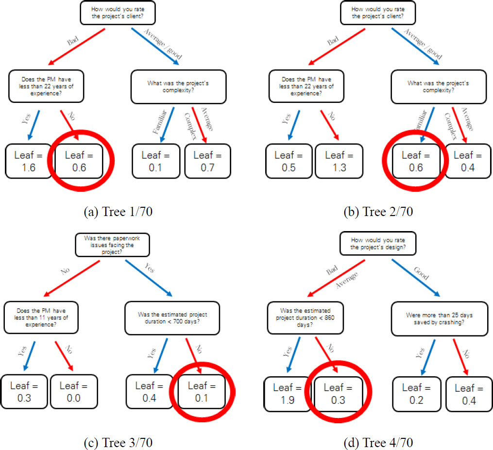
Case illustration trees.
A project from the testing dataset is chosen at random, and its parameters are shown in Table 4.
| Project Parameter | Value |
|---|---|
| Estimated duration | 900 |
| Supplier average delay | 30 |
| Subcontractor average delay | 30 |
| PM years of experience | 25 |
| Design quality (0 – 1 – 2) | 2 |
| Consultant Performance (0 – 1) | 0 |
| Percentage subcontracted | 60 |
| Project complexity (0 – 1 – 2) | 2 |
| Issues faced (0 – 1) | 1 |
| Days saved by crashing | 60 |
| Client performance (0 – 1 – 2) | 0 |
| Project delay percentage | 19 |
The test observation was propagated through all 70 trees to obtain the predicted delay. For the first four trees (Fig. 3), the leaf outputs were 0.6%, 0.6%, 0.1%, and 0.3%, respectively. The ensemble prediction is the sum of the leaf values returned by each tree. For this case, summing the contributions from trees 1–70 produced a predicted delay of 25% of the planned duration, as shown in Eq. (1). The observed delay for this project was 19%, so the residual for this example is 6 percentage points.
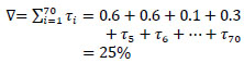
where ∇ is the predicted project delay and τi denotes the leaf contribution (in percent) from tree i
2. RESULTS AND DISCUSSION
Model performance was assessed using repeated randomized train/test partitions and reported as the mean across runs to reduce sampling variability. The model yields three complementary outputs of operational value to practitioners: a point estimate, an empirically derived 90% prediction interval conveying uncertainty around that estimate and enabling probabilistic interpretation of expected delay magnitude, and the top three contributing factors that drive the prediction. Together, these outputs enable project teams to quantify expected schedule risk, prioritize mitigation efforts on the most influential drivers, and make informed scheduling or contractual decisions before construction begins.
On average, the tuned XGBoost model demonstrated strong predictive performance on the available dataset. Reported metrics are averages over 1,000 randomized train/test partitions (75% train / 25% test) with 10-fold cross-validation used during training. The tuned XGBoost regression model achieved a Mean Absolute Error (MAE) of 4.36 percentage points, indicating that predicted delay percentages deviated from observed delays by approximately 4.36 points on average. The overall percentage error was 24%. Goodness-of-fit was high, with R2 = 79.6% (adjusted R2 = 74.3%), showing that the model explains the majority of variance in measured delay percentages after accounting for model complexity. The distribution of MAE across the 1,000 repeated evaluations indicates the stability of predictive performance across different randomized train–test partitions. The reported MAE of 4.36 percentage points should therefore be interpreted as the average performance across repeated evaluations rather than as the result of a single favorable split. The corresponding uncertainty summary is reported in the Abstract as a mean MAE of 4.36 ± 0.48 percentage points, with a 95% confidence interval of 3.42–5.30 percentage points.
For the 15 test projects with observed and predicted delay percentages supplied for this study, the Root Mean Squared Error (RMSE) was 4.82 percentage points, and the MAE was 4.07 percentage points. For context, a no-delay baseline, which predicts zero overrun for every project, had an MAE of 15.07 percentage points on the same test set. These single-test-set results are distinct from the averages across repeated partitions reported above.
The observed predictive performance can be attributed to the ability of the boosted-tree ensemble to capture nonlinear relationships and interactions among the selected project variables while progressively correcting residual prediction errors. In addition, the use of shallow trees, cross-validation-based hyperparameter tuning, row and feature subsampling, and L1 regularization helped control model complexity and reduce overfitting. The compact predictor set, selected from recurrent delay factors identified in the literature, may also have contributed to the model’s ability to achieve good predictive performance with the available dataset.
The standard deviation of prediction errors was 4.6%, which, together with the mean absolute error, indicates a typical distribution of residuals and was used to develop empirical prediction intervals for individual forecasts. The obtained standard deviation falls within the lower range for values found in similar studies, ranging from 3.9 [29] to 11.1 [37]. All reported figures are averages computed over the repeated cross-validation and hold-out evaluations. The results of the model output on the test set are shown in Fig. (4) and are compared to the actual delay percentages, including the 90% prediction interval.
In Figure 4, one can see that only one model prediction out of the 15 test-set projects fell outside of the 90% prediction interval. This shows that the model is well-calibrated and can capture the central tendency and uncertainty of delay outcomes with reliability, while accounting for residual variability. Prediction accuracy naturally varies across individual projects, particularly when atypical, high-impact factors (outliers) are present. However, such cases were infrequent in the used sample. Given the observed standard deviation of prediction errors and the model’s calibration, a user can expect accurate and informative delay estimates for most projects, thus making the tool useful for early risk assessment and schedule planning.
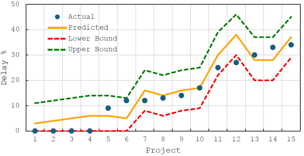
Predicted vs. observed delay %.
Although the tuning procedure evaluated combinations of the principal hyperparameters, the subsequent one-dimensional refinement did not exhaustively explore all possible higher-order interactions. More extensive joint optimization, such as Bayesian optimization or a larger randomized search, could be examined in future work. This limitation does not alter the interpretation of the present model as a practically optimized predictive model rather than an exhaustive analysis of the XGBoost hyperparameter space.
2.1. Interpretation of Predictor Effects
One predictor variable was removed at a time from the model input to evaluate its effect on the accuracy of the model by observing the change in mean absolute error on the test set. By examining Fig. (5), one can see how much the mean absolute error increased when each predictor factor was removed from the model input. The client (owner) performance and legal issues are identified as primary drivers of delay in the sample. Design quality and the Project Manager’s (PM) experience ranked third and fourth, respectively. These findings indicate that pre-project governance, client clarity and commitment, and design robustness are essential for reducing schedule risk. Supplier and subcontractor delay metrics and time savings from crashing activities proved to be less influential predictors for schedule delays. Because XGBoost captures nonlinear relationships and interactions among predictors, the reported importance values represent their relative contribution to predictive performance rather than fixed marginal effects or regression coefficients. Because the leave-one-predictor-out analysis evaluates the change in predictive error when a variable is omitted, the resulting ranking should be interpreted as predictive importance within the present dataset rather than as evidence of causal effects.
The leave-one-predictor-out analysis is a descriptive assessment of predictive importance; no inferential significance tests were used to assess model performance or predictor importance.
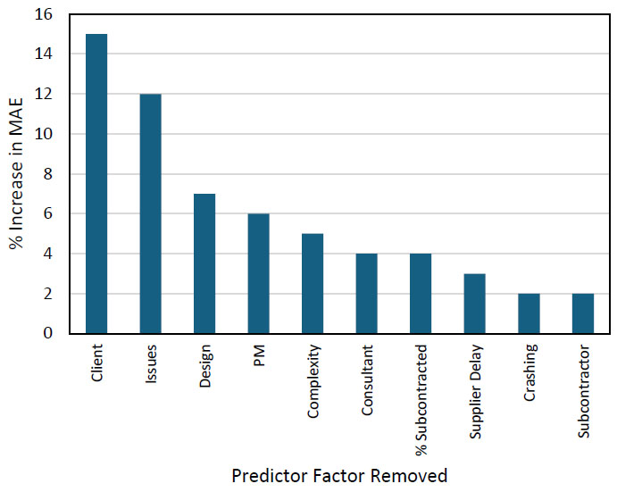
Predictor factor importance.
2.2. Practical implications
By requiring only eleven readily obtainable pre-project inputs, the model provides a practical decision support tool for project managers to estimate expected delay magnitude and its uncertainty before construction initiation. Outputs can inform mitigation strategies (e.g., contractual safeguards, design improvements, staffing or procurement interventions), scheduling adjustments, or negotiation of completion dates. While the model requires eleven user inputs, users may omit an input and still obtain an estimate, but predictive accuracy declines as more values are left unspecified. The highest-ranked predictors can be used as indicators of areas that may warrant additional managerial attention, risk review, or mitigation planning; however, their predictive importance should not be interpreted as evidence that modifying an individual factor will necessarily produce a causal reduction in project delay.
The following workflow describes how project teams can apply the pre-construction XGBoost delay model in practice to produce an adjusted completion forecast and prioritize mitigation actions. It assumes the user has a baseline schedule (e.g., CPM/Primavera) and can provide the simple pre-project inputs required by the tool.
- Prepare baseline schedule: Compute the project’s estimated duration using standard scheduling tools (e.g., CPM/Primavera). Use this duration as the model’s “estimated duration” input.
- Collect pre-project inputs: Gather the required pre-start predictors for the project: estimated duration (days), percentage of late supplier deliveries, percentage of subcontractor tasks delayed, project-manager years of experience, percentage of project subcontracted, days expected to be saved by crashing, design quality (0 poor / 1 average / 2 good), consultant performance (0 poor / 1 good), project complexity (0–2), presence of legal/ municipality issues (0/1), and client/owner performance (0–2). Use the same ordinal encodings as specified in Table 1.
- Encode and validate inputs: Convert categorical/ordinal answers to numeric codes; verify numeric ranges and plausibility (e.g., percentage fields between 0–100). Correct or query obvious data entry errors before running the model.
- Run the model: Input the eleven values into the tool. The model returns: (a) a point estimate of expected delay (percentage of estimated duration), (b) a 90% empirical prediction interval, and (c) the top three contributing factors ranked by their impact on the forecast.
- Interpret and integrate outputs: Convert the predicted delay percentage to days and add to the baseline CPM estimate to obtain an adjusted expected completion date. Use the 90% interval to express forecast uncertainty to stakeholders. Use the ranked factors to prioritize mitigation actions (e.g., strengthen client payment/ communication protocols, accelerate permit resolution, improve design completeness, and assign a more experienced PM).
- Decision and mitigation actions: Based on the adjusted schedule and top risk drivers, implement targeted mitigations (contract clauses, early procurement, design reviews, PM reassignment, contingency budgeting) or renegotiate milestones/contract terms if residual risk remains unacceptable.
In the case of large predicted delays or unusually wide prediction intervals, these often indicate either (a) true high risk (e.g., anticipated legal disputes, major financing uncertainty) or (b) an input configuration outside the model’s training distribution. In these cases, the user/project manager should: (1) treat the forecast as an alert requiring qualitative review; (2) inspect and verify inputs for errors; (3) perform a root-cause assessment focused on the top reported factors; and (4) consider bespoke risk analysis (detailed risk workshop, expert review, scenario planning) rather than relying solely on the model output.
2.3. Comparison with Prior Work
To show how this study advances the literature, the results are compared with those of previous studies that developed models to predict scheduling delays using large feature sets that include between 30 and 60 factors. Table 5 shows that this study advances the literature by (1) producing a regression model that estimates delay magnitude rather than class membership, and (2) achieving substantial explanatory power with a compact feature set (eleven predictors), thereby enhancing operational usability. The reported performance values are included for contextual completeness only. Because previous studies predominantly employ classification outcomes, whereas the present study employs regression, their classification accuracies are not directly comparable with the MAE and R2 reported herein and should not be interpreted as evidence of relative predictive superiority.
The analysis of key input factors aligns with findings from previous studies: owner/client performance and legal/permit issues being the two strongest predictors of schedule delays, followed by design quality and project manager’s experience. Project complexity, consultant performance, and the share subcontracted had a moderate effect on the accuracy of the model, whereas supplier delays, days saved by crashing, and the proportion of subcontractor tasks experiencing delays had minimal effect.
It is worth noting that although many previous studies identified project manager’s experience as the single most influential factor, this factor ranked fourth in this model. This discrepancy is likely due to the use of years of experience of the project manager as a coarse operationalization to reflect the PM’s true competence. A more granular representation of managerial competence, such as qualifications, demonstrated past performance, or firm-level process metrics, would likely capture this factor’s influence more accurately and could change the relative ranking of the predictors.
3. LIMITATIONS
Although the dataset used has a sample size equal to or greater than those reported in similar studies, a larger and more diverse dataset could improve the model’s generalizability and robustness. The data contributed by surveyed firms were not uniform, which may have introduced bias toward certain dominant contributors. Interacting project constraints and compound risks can disproportionately affect schedule sensitivity and contribute to larger, non-uniform prediction errors [40].
Some predictors (e.g., project manager competence) were represented by single coarse measures (years of experience). Incorporating richer measures of managerial qualifications, track record, and firm-level practices could increase explanatory power.
Data were collected for completed projects with respondents asked to report values they would have known prior to construction. Although respondents were instructed to provide pre-project values, retrospective reporting may introduce recall bias or post-hoc rationalization. Prospective data collection and validation on new projects is recommended.
CONCLUSION AND RECOMMENDATIONS
This study developed and validated an XGBoost-based regression model that estimates the magnitude of building construction schedule delays prior to project commencement using eleven pre-project predictors. The tuned model achieved an adjusted R2 of 74.3% and a mean absolute error of 4.36 percentage points across repeated evaluations, demonstrating that a parsimonious set of readily obtainable inputs can produce actionable, probabilistically calibrated delay estimates. The deployed tool returns a point estimate, a 90% prediction interval, and the top contributing factors for each prediction, offering practical decision support for early risk assessment and mitigation planning.
The model presented a regression approach, rather than classification, for predicting delay magnitude, filling a gap in existing literature. It demonstrated that reliable pre-project estimates can be obtained from a compact, operationally practical feature set, reducing data burden for practitioners. The model delivers interpretable outputs (prediction interval and ranked factor importance) that enable project managers to identify dominant risk drivers and prioritize mitigation actions before construction begins. In practice, users can combine traditional duration estimates (e.g., CPM, Primavera) with the model’s delay prediction to obtain an improved forecast of project completion and to inform decisions such as design improvements, contractual safeguards, resource allocation, or even project acceptance.
Current and Future Developments
The model was developed on building construction projects; extending its applicability to infrastructure, industrial, or other project classes requires additional, domain-diverse training data and potential feature adaptation. Future work should (1) expand the dataset across more projects and diverse geographic and project contexts, (2) enrich predictor detail, especially regarding project manager competence and contractual/financial variables, (3) carry out prospective validation on new projects to assess real-time predictive performance, (4) adapt and evaluate the model for non-building project classes, and (5) evaluate gradient-boosting variants (CatBoost, LightGBM), which comparative studies indicate can offer competitive performance, in future external validations [41]. Future research should benchmark the proposed approach against simpler and alternative regression models, including linear and regularized regression, shallow tree-based models, Random Forest, SVR, CatBoost, and LightGBM, using identical predictors, data partitions, tuning procedures, and evaluation criteria.
AUTHORS’ CONTRIBUTIONS
The authors confirm their contributions to the paper as follows: C.A.S., R.A.: Study conception and design; J.N.: Data collection; J.N., C.A.S., R.A.: Analysis and interpretation of results; J.N.and C.A.S.: Draft manuscript. All authors reviewed the results and approved the final version of the manuscript.
LIST OF ABBREVIATIONS
| AI | = Artificial Intelligence |
| CI | = Confidence Interval |
| CPM | = Critical Path Method |
| GDP | = Gross Domestic Product |
| L1 | = L1 (absolute-value) regularization |
| LightGBM | = Light Gradient Boosting Machine |
| MAE | = Mean Absolute Error |
| ML | = Machine Learning |
| MS | = Microsoft (MS Project) |
| PERT | = Program Evaluation and Review Technique |
| PM | = Project Manager |
| PMBOK | = Project Management Body of Knowledge |
| PNET | = Probabilistic Network Evaluation Technique |
| R2 | = Coefficient of Determination |
| RMSE | = Root Mean Squared Error |
| SVR | = Support Vector Regression |
| U.S. | = United States |
| XGBoost | = Extreme Gradient Boosting |
AVAILABILITY OF DATA AND MATERIALS
The underlying project-level dataset contains commercially sensitive information provided by participating firms. An anonymized version of the dataset (firm identifiers and any sensitive fields removed) and the code used for preprocessing, model training, and figure generation are available from the corresponding author upon reasonable request.
ACKNOWLEDGEMENTS
Declared none.