All published articles of this journal are available on ScienceDirect.

Prediction of Thermal Stresses During the Construction of Massive Monolithic Foundation Slabs Using Temperature Monitoring Data
Abstract
Introduction
Thermal cracking during the early-age hardening of massive monolithic foundation slabs poses significant risks to structural durability and integrity. Traditional analytical methods for assessing thermal stresses rely on simplifying assumptions, such as a parabolic temperature distribution, while numerical methods like the finite element method (FEM) are computationally intensive and sensitive to uncertain boundary conditions.
Materials and Methods
This study proposes a novel methodology integrating real-world temperature monitoring data with machine learning to predict thermal stresses at three characteristic points (bottom, middle, and top) across the slab thickness. A comprehensive dataset of 717,360 records was collected using FEM-based numerical experiments, considering variations in concrete class, slab thickness, curing time, heat release kinetics, and ambient conditions. The CatBoost gradient boosting algorithm was selected for its robustness to multicollinearity and its ability to model complex, nonlinear relationships.
Results
The developed model demonstrated exceptional predictive accuracy, with a coefficient of determination (R2) exceeding 0.99 for all stress components and mean absolute errors (MAE) of 0.130 MPa, 0.383 MPa, and 0.060 MPa for the bottom, middle, and top surfaces, respectively. Feature importance analysis revealed that the heat release rate (99%) and curing time (96%) predominantly influence bottom surface stresses, while the central temperature (94%) governs stresses at the slab’s mid-depth.
Discussion
Validation against independent experimental data confirmed the model's high fidelity up to the point of crack formation. The proposed approach implicitly accounts for the time-dependent evolution of concrete's elastic modulus through temperature–time parameters, overcoming key limitations of existing analytical solutions.
Conclusion
The proposed methodology enables rapid, near-real-time assessment of thermal stresses directly from in-situ monitoring data, providing a powerful and computationally efficient tool for early-age crack risk management during the construction of massive foundation slabs.
1. INTRODUCTION
The formation of temperature cracks during construction is one of the most common problems encountered in massive monolithic concrete structures under real-world conditions. Completely crack-free structures are extremely rare in practice. During the early stages of concrete hardening, the exothermic hydration reaction of cement causes intense heat release, leading to an increase in temperature within the structure. As the outer surfaces cool, a temperature gradient develops, causing the central zones of the concrete to remain warmer than the surface layers [1, 2].
Uneven thermal expansion of various zones of a concrete element leads to the development of internal stresses. Thermal cracks form when tensile stresses at the surface exceed the ultimate tensile strain capacity or early tensile strength of the concrete. Additional tensile stresses may arise due to early restraint caused by autogenous shrinkage of the concrete. Early cracking depends on a variety of factors, including the composition of the concrete mix, the conditions of heat exchange with the environment, the rate of cement hydration, and the curing parameters of the material [3].
Thermal cracking reduces the strength, durability, and water resistance of concrete structures, facilitates the penetration of moisture and aggressive environments, and thereby accelerates material degradation. This necessitates the assessment of the thermal stresses that arise during the curing of massive monolithic foundation slabs. One of the most versatile tools for such analysis is the finite element method (FEM). This method is widely used to analyze the temperature–stress state during construction and allows for consideration of complex structural geometry, transient heat transfer, and the phased nature of concreting [4].
During the curing process, concrete undergoes changes in its physical and mechanical properties. Characteristics such as thermal conductivity and specific heat capacity typically undergo insignificant changes at an early stage. At the same time, the mechanical properties of concrete (modulus of elasticity, compressive strength, and tensile strength) change significantly during the first 28 days of curing. Ignoring the evolution of these properties can lead to significant errors in assessing the stress–strain state of a structure, since accounting for changes in the modulus of elasticity affects not only the quantitative but also the qualitative characteristics of stress distribution [5].
Based on FEM, many software packages have been implemented, such as ABAQUS, ANSYS, ELCUT, and Midas Civil, allowing step-by-step assessment of temperature fields and stresses in massive concrete structures [6-9]. For example, W. Cui et al. [10] developed a thermomechanical model using ABAQUS and the XFEM method, accounting for changes in the mechanical properties of concrete over time. Field tests conducted on a massive concrete pier demonstrated good agreement between the calculated and experimental data: the maximum temperature obtained in the calculation was 61.73 °C, while the measured value reached 62.75 °C.
The authors of [11] proposed a method for calculating the temperature field in massive concrete, based on an improved kinetic model of cement hydration that combines neural networks to determine the model parameters and a Taylor expansion to describe exothermic reactions. Validation of the method using the example of a 5.5-meter-thick foundation slab for a high-rise building demonstrated its advantages over traditional empirical relationships. G. Liu et al. [12] developed an integrated FEM-XFEM model for analyzing crack formation in concrete dams, taking into account temperature and mechanical factors. Experimental verification showed that the discrepancy between the calculated and actual number of cracks does not exceed 10%. A number of studies [13-16] have also demonstrated the high accuracy of FEM approaches in the analysis of temperature fields and stresses in massive concrete slabs, tunnels, pylons, and prestressed elements, with discrepancies between calculated and experimental temperature data typically not exceeding 1–3%.
Despite its high accuracy, the finite element method has a number of drawbacks. A significant limitation is the difficulty of specifying boundary and initial conditions, which can vary significantly under real-world construction conditions (ambient temperature, wind speed, heat transfer coefficients, solar radiation, etc.). Even minor discrepancies between calculated and actual temperature fields can lead to significant errors in thermal stress assessment. Therefore, the development of stress assessment methods based on actual measured temperatures in a structure is of particular interest.
For the engineering assessment of thermal stresses in massive monolithic foundation slabs, the analytical expression (Eq. 1) is widely used [17]:
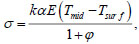
where σ are the temperature stresses; k = 0.833 is the coefficient of deformation restraint; α is the concrete linear thermal expansion coefficient; E is the modulus of elasticity of concrete; φ is the creep coefficient; Tmid - Tsurf and is the temperature difference between the middle and the surface of the slab.
This formula has a number of significant limitations. First, it assumes identical heat exchange conditions on the upper and lower surfaces of the slab, which is practically impossible under real construction conditions. Second, the expression does not take into account the history of changes in the concrete modulus of elasticity up to the given moment in time, which, as shown in a number of studies [18, 19], has a significant impact on the formation of the stress–strain state. The authors of the work [20] analyzed the dependence of temperature stresses on changes in the thermal and mechanical properties of concrete (coefficient of thermal expansion, modulus of elasticity, shrinkage, etc.) at an early age and showed that this factor significantly affects the accuracy of analytical models. Third, formula (1) is derived based on the hypothesis of a parabolic temperature distribution across the thickness of the slab, which poorly describes the real temperature fields in thick slabs.
As part of the development of traditional analytical approaches, reference [21] also proposes a simplified analytical method for assessing thermal stresses in massive monolithic foundation slabs based on temperatures measured at three characteristic points along the thickness of the structure: on the lower surface, in the middle of the slab, and on the upper surface. Unlike the classical expression (1), this approach allows for the difference in heat exchange conditions on the upper and lower surfaces of the slab to be taken into account, significantly increasing the accuracy of thermal stress calculations compared to models based solely on the temperature difference between the center and the surface.
The analytical relationships obtained in [21] were verified by comparing them with the results of finite element analysis and experimental data presented in the works of other researchers. It was shown that for slabs up to 2 m thick, the error in determining the maximum tensile stresses at characteristic points does not exceed 10%, and the discrepancy from the FEM results for stresses at the center of the slab is approximately 0.4%.
However, the proposed method has a number of limitations. Specifically, it is based on the hypothesis of a parabolic temperature distribution across the slab thickness, which limits its applicability for massive foundation slabs (over 2 m), where actual temperature fields can deviate significantly from the parabolic shape. Furthermore, the analytical nature of the formulas does not allow full consideration of the complex evolution of concrete’s thermal and mechanical properties under transient curing and operating conditions, limiting the accuracy of stress assessments.
In recent years, machine learning methods have been increasingly used to predict thermal effects and the risk of early-age cracking in massive concrete structures. For example, a comprehensive approach to assessing the potential for thermal cracking in the early stages of concrete hardening in bridge supports using machine learning methods was proposed in [22]. The authors developed models for predicting the maximum potential for thermal cracking and the time of its possible manifestation based on a dataset generated using the EACTSA software package. It was noted that, compared to traditional analytical and numerical methods, the proposed machine learning models provide significantly higher computational efficiency and can be used to quickly optimize geometric parameters, select formwork removal times, and control the temperature regime, reducing the risk of early-age thermal cracking.
Despite the growing interest in the application of machine learning methods to predict the behavior of reinforced concrete structures, existing research in this area has mainly focused on predicting the strength properties of elements with various configurations. For example, authors of paper [23] developed artificial intelligence models to assess the strength of reinforced concrete beams as a replacement for empirical and semi-empirical prediction models. A similar task was addressed in [24, 25] for eccentrically compressed concrete-filled steel tubular columns using CatBoost algorithms and other machine learning methods.
Regarding the application of machine learning specifically to massive concrete structures, the recent work by Van Tran et al. [26] deserves special attention. In this paper, a hybrid ensemble ML framework (XGB-CatBoost-Lasso) is proposed for predicting the temperature evolution in massive concrete with pipe cooling, based on data obtained from real wind turbine foundation construction projects. The authors showed that the cooling system parameters have a dominant influence on the concrete temperature regime, and the use of machine learning methods allows for real-time temperature monitoring and adaptive control of the cooling process. Work [27] also focuses on predicting temperature fields; the results confirm the suitability of ML models for reliably predicting the thermal response.
Thus, an analysis of existing publications reveals that, despite the active development of ML approaches in structural mechanics, most studies use machine learning models primarily to predict temperature or strength characteristics without a direct connection to actual measured data on the structural condition. This highlights a scientific gap: the lack of integration of real-world temperature monitoring data with intelligent models for the highly accurate assessment of thermal stresses at characteristic points in massive monolithic slabs. Addressing this gap and developing a practice-oriented methodology for assessing thermal stresses based on monitoring data and machine learning methods is the goal of this study.
The proposed methodology aims to eliminate the limitations of traditional analytical formulas, takes into account the differences in heat exchange conditions on the surfaces of the structure and the evolution of the mechanical properties of concrete over time, which ensures a more accurate and practice-oriented assessment of thermal stresses during the construction of massive monolithic foundation slabs.
2. MATERIALS AND METHODS
The subject of the study is a massive monolithic foundation slab being constructed under real-world construction conditions. During the concrete curing process, intense heat generation occurs within the structure due to cement hydration. This leads to the formation of an uneven temperature field across the slab’s thickness and the occurrence of thermal stresses.
The results of a series of numerical experiments assessing thermal stresses were used as input data for the machine learning models. The model's input parameters were temperatures at three characteristic points: Tbot on the bottom surface of the slab; Tmid at the slab’s mid-depth; and Tup on the upper surface of the slab. This arrangement of sensors allows obtaining the minimum necessary information about the temperature distribution across the thickness of the structure and determining the temperature gradients that influence the formation of the stress state.
Additional input parameters were also introduced: concrete curing time t in days; concrete compressive strength class B according to Russian standard GOST 18105-2018; slab thickness h in meters; and a heat release kinetics parameter rate, which takes the values 1 for rapid-hardening concrete, 2 for normal-hardening concrete, and 3 for slow-hardening concrete.
Output parameters were the stress on the lower surface of the slab σbot, the stress at the mid-thickness of the slab σmid, and the stress on the upper surface of the slab σup in MPa.
When forming the training dataset, the concrete class varied from B20 to B50 in steps of 5 MPa. The slab thickness h varied from 0.75 to 3 m in steps of 0.25 m. The heat transfer coefficient hup on the upper surface of the slab took values from 2 to 30 W/(m2 ∙ °C) in steps of 4 W/(m2 ∙ °C). The ambient temperature T∞ varied from 5 to 35 °C in steps of 5 °C. The calculation of temperature fields and stresses was performed over a time range from 0 to 30 days. The results were written into the training dataset at intervals of 0.5 days. For each set of values, [B h hup T∞ rate] the values [Tbot Tmid Tup σbot σmid σup] were determined by calculating the temperature fields and stresses using the method given in [28]. The values [Tbot Tmid Tup], along with the parameters t, B, h, were written in columns corresponding to the input parameters of the model, and the values [σbot σmid σup] were placed in columns corresponding to the output parameters. When calculating the temperature field, the heat release function was taken in the form [29] (Eq. 2):
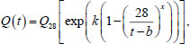
Where Q28 is the integral heat release of 1 m3 of concrete by the age of 28 days, k and x are the coefficients determining the kinetics of heat release of concrete, t is the time in days, b and is the induction period in days.
The values of thermophysical characteristics adopted in the calculation of the temperature field are given in Table 1.
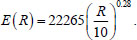
The cubic compressive strength of concrete was determined as a function of its equivalent age (Eq. 3):
| Material | Density ρ (kg/m3) | Thermal Conductivity Coefficient λ (W/(m∙°С)) |
Specific Heat Capacity c (J/(kg∙°C)) |
|---|---|---|---|
| Concrete | 2400 | 2.67 | 1000 |
| Soil | 2000 | 1.62 | 2250 |
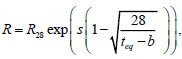
Where s is a coefficient depending on the kinetics of concrete strength gain, R28 is the cubic compressive strength of concrete at the age of 28 days, and teq is the equivalent age of concrete, determined by the integral (Eq. 4):
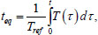
Where Tref = 20 ° C is the standard condition temperature, T(τ) and is the temperature of concrete at the age τ.
The modulus of elasticity of concrete at an equivalent age of at least 0.5 days was determined using the formula [30] (Eq. 5):
The values of heat generation parameters and strength gain kinetics used in the calculation, depending on the concrete class and its category by hardening rate, are given in Table 2.
| Parameter | k | x | s | Q28 (MJ/m3) | b (days) | R28 (MPa) |
|---|---|---|---|---|---|---|
| Rapid hardening (rate = 1) | 0.14 | 0.4 | 0.2 | 130 + 3 ∙(B – 25) | 0.167 | B +12 |
| Normal hardening (rate = 2) | 0.19 | 0.51 | 0.35 | |||
| Slow hardening (rate = 3) | 0.24 | 0.62 | 0.5 |
Table 3 shows a portion of the analyzed dataset. The total number of numerical experiments was 11,760. The dataset size was 11,760 × 61 = 717,360 rows, where 61 is the number of time points.
| - | Input Parameters | Output Parameters | ||||||||
|---|---|---|---|---|---|---|---|---|---|---|
| No. | Tbot (°C) | Tmid (°C) | Tup (°C) | t (days) | B (MPa) | h (m) | rate | σbot (MPa) | σmid (MPa) | σup (MPa) |
| 1 | 5 | 5 | 5 | 0 | 20 | 0.75 | 1 | 0 | 0 | 0 |
| 2 | 16.62149 | 27.8569 | 26.34837 | 0.5 | 20 | 0.75 | 1 | 0 | 0 | 0 |
| 3 | 19.83056 | 30.40945 | 29.38324 | 1 | 20 | 0.75 | 1 | -0.14973 | 0.056754 | -0.06045 |
| 4 | 21.0141 | 29.77187 | 28.65189 | 1.5 | 20 | 0.75 | 1 | -0.60061 | 0.145894 | 0.058365 |
| 5 | 21.42112 | 28.51148 | 27.12443 | 2 | 20 | 0.75 | 1 | -1.05346 | 0.222462 | 0.222953 |
| 6 | 21.41961 | 27.13235 | 25.51349 | 2.5 | 20 | 0.75 | 1 | -1.44321 | 0.287235 | 0.366313 |
| 7 | 21.18725 | 25.79248 | 24.01039 | 3 | 20 | 0.75 | 1 | -1.76317 | 0.341879 | 0.477289 |
| 8 | 20.82452 | 24.54438 | 22.65878 | 3.5 | 20 | 0.75 | 1 | -2.02194 | 0.387894 | 0.559451 |
| 9 | 20.39131 | 23.40146 | 21.45722 | 4 | 20 | 0.75 | 1 | -2.2307 | 0.426692 | 0.61888 |
| 10 | 19.92403 | 22.36181 | 20.39105 | 4.5 | 20 | 0.75 | 1 | -2.39959 | 0.459531 | 0.661064 |
| 11 | 19.44497 | 21.41778 | 19.44303 | 5 | 20 | 0.75 | 1 | -2.53689 | 0.487472 | 0.69033 |
| 12 | 18.96774 | 20.56001 | 18.59691 | 5.5 | 20 | 0.75 | 1 | -2.64914 | 0.511387 | 0.709943 |
| … | … | … | … | … | … | … | … | … | … | … |
| 717348 | 66.9232 | 69.26768 | 37.64744 | 24 | 50 | 3 | 3 | -3.83489 | -1.72061 | 7.650354 |
| 717349 | 66.73431 | 68.76469 | 37.59947 | 24.5 | 50 | 3 | 3 | -3.92345 | -1.65463 | 7.496323 |
| 717350 | 66.54192 | 68.27147 | 37.55279 | 25 | 50 | 3 | 3 | -4.00742 | -1.59046 | 7.344391 |
| 717351 | 66.34643 | 67.78791 | 37.50738 | 25.5 | 50 | 3 | 3 | -4.087 | -1.52806 | 7.194579 |
| 717352 | 66.14823 | 67.3139 | 37.46318 | 26 | 50 | 3 | 3 | -4.16237 | -1.46739 | 7.046903 |
| 717353 | 65.94767 | 66.84929 | 37.42016 | 26.5 | 50 | 3 | 3 | -4.23372 | -1.4084 | 6.901373 |
| 717354 | 65.74508 | 66.39395 | 37.37829 | 27 | 50 | 3 | 3 | -4.30122 | -1.35104 | 6.757992 |
| 717355 | 65.54076 | 65.94771 | 37.33751 | 27.5 | 50 | 3 | 3 | -4.36505 | -1.29528 | 6.616759 |
| 717356 | 65.335 | 65.51043 | 37.29781 | 28 | 50 | 3 | 3 | -4.42537 | -1.24107 | 6.477669 |
| 717357 | 65.12805 | 65.08194 | 37.25913 | 28.5 | 50 | 3 | 3 | -4.48234 | -1.18836 | 6.340712 |
| 717358 | 64.92016 | 64.66207 | 37.22146 | 29 | 50 | 3 | 3 | -4.5361 | -1.13711 | 6.205875 |
| 717359 | 64.71155 | 64.25065 | 37.18475 | 29.5 | 50 | 3 | 3 | -4.5868 | -1.08728 | 6.073143 |
| 717360 | 64.50243 | 63.84752 | 37.14898 | 30 | 50 | 3 | 3 | -4.63457 | -1.03883 | 5.942498 |
In traditional engineering methods, thermal stresses in massive concrete structures are estimated using simplified analytical relationships based on the temperature difference between the center and the surface of the structure. This study proposes an improved approach that takes into account the temperature at three characteristic points of the structure: the bottom surface, the mid-depth, and the top surface of the slab. To improve the quality of the models, a correlation analysis was carried out for all variables, and heatmaps of linear dependencies between input and output parameters were constructed.
To analyze the correlation between the input characteristics and stresses at three characteristic points, the Pearson correlation coefficient was used, and the influence of temperature distribution, curing time, and concrete properties on the stress state of the slab was studied. Machine learning models based on decision trees were selected to solve the problem. The CatBoost regression was chosen due to its robustness to multicollinearity, ability to model nonlinear relationships, and high forecasting accuracy. Stratified splitting into training and test sets was used at the level of independent design cases, not at the level of time points. That is, all time points from a single FEM calculation (one set of parameters: concrete grade, thickness, curing rate, etc.) were entirely included in either the training or test sample. This prevents adjacent time steps from the same scenario from being included in both the train and test samples.
To assess the quality and stability of the constructed forecasting models, graphs of residuals over time were constructed for the stress components σbot, σmid, and σup. The residuals were determined as the difference between the actual and predicted stress values. The analysis was performed on a test sample, with the concrete curing time plotted on the abscissa and the residual values on the ordinate.
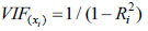
Variance Inflation Factor (VIF) analysis was performed to identify multicollinearity of input parameters. The calculation method is an inversely proportional relationship between the threshold values of quantitative estimates of the degree of multicollinearity for the selected data set and the corresponding coefficients of determination. By selecting feature xi, where i = {1:7}, the remaining features act as independent features, thereby examining the dependence of the selected feature on the remaining features and determining how much better this feature is relative to the others. The VIF values are calculated using the formula (Eq. 6):
 = 0 is interpreted as a complete absence of a relationship; when
= 1 shows the presence of a strong linear relationship. When
= 1, VIF is equal to infinity. Threshold values: VIFxi<5 show the moderate relationship; 5≤VIFxi<10 show the high correlation; VIFxi≥10 is the critical multicollinearity.
= 0 is interpreted as a complete absence of a relationship; when
= 1 shows the presence of a strong linear relationship. When
= 1, VIF is equal to infinity. Threshold values: VIFxi<5 show the moderate relationship; 5≤VIFxi<10 show the high correlation; VIFxi≥10 is the critical multicollinearity.
Additionally, the importance of features was analyzed using the SHAP analysis method based on the theory of the Shapley vector [31]. The impact of each input feature on the performance of the forecasted values in terms of depth and direction was assessed.
To tune the model's hyperparameters, a grid search with 5-fold cross-validation was conducted to find the optimal parameters. Table 4 presents the key hyperparameters for the CatBoost model.
| No. | Parameter | Value |
|---|---|---|
| 1 | depth | 4, 6, 8 |
| 2 | learning_rate | 0.03, 0.05, 0.1 |
| 3 | iterations | 500, 1000 |
Model quality is assessed for each parameter combination across all cross-validation splits. This method takes some time, as we have 18 parameter combinations (3 x 3 x 2) and 5-fold cross-validation, resulting in a total of 90 executions of the algorithm.
To assess the accuracy of a specific combination of parameter values for the constructed models, the average cross-validity value for each parameter combination was calculated. The dataset was split into training and test sets at an 80/20 ratio, with 15% of the training set serving as the validation set.
3. RESULTS
The statistical characteristics of the original dataset are presented in Table 5. This table also shows the ranges of variation of the input and output parameters. Key indicators include sample size, sample mean, variance, and extreme values of the variables.
| - | Tbot | Tmid | Tup | t | B | h | rate | σbot | σmid | σup |
|---|---|---|---|---|---|---|---|---|---|---|
| count | 717360 | 717360 | 717360 | 717360 | 717360 | 717360 | 717360 | 717360 | 717360 | 717360 |
| mean | 37.21 | 40.83 | 26.65 | 15.0 | 35.0 | 1.88 | 2.00 | -2.92 | -0.34 | 1.24 |
| std | 13.11 | 16.90 | 12.43 | 8.8 | 10.0 | 0.72 | 0.82 | 2.80 | 1.17 | 2.92 |
| min | 5.00 | 5.00 | 5.00 | 0.0 | 20.0 | 0.75 | 1.00 | -12.25 | -5.88 | -10.27 |
| 25% | 27.74 | 28.50 | 16.74 | 7.5 | 25.0 | 1.25 | 1.00 | -4.69 | -0.99 | -0.44 |
| 50% | 37.21 | 39.82 | 26.38 | 15.0 | 35.0 | 1.88 | 2.00 | -2.73 | -0.10 | 1.08 |
| 75% | 46.77 | 52.18 | 35.60 | 22.5 | 45.0 | 2.50 | 3.00 | -1.05 | 0.44 | 2.97 |
| max | 72.90 | 103.46 | 83.43 | 30.0 | 50.0 | 3.00 | 3.00 | 6.46 | 2.95 | 12.57 |
Since machine learning is essentially a multivariate interpolation, reliable model performance can only be guaranteed within the limits of input parameter variation in the training dataset. The minimum and maximum input parameter values listed in Table 5 cover the range of the most common characteristics of massive monolithic foundation slabs.
Figure 1 shows the correlation matrix for all model parameters.
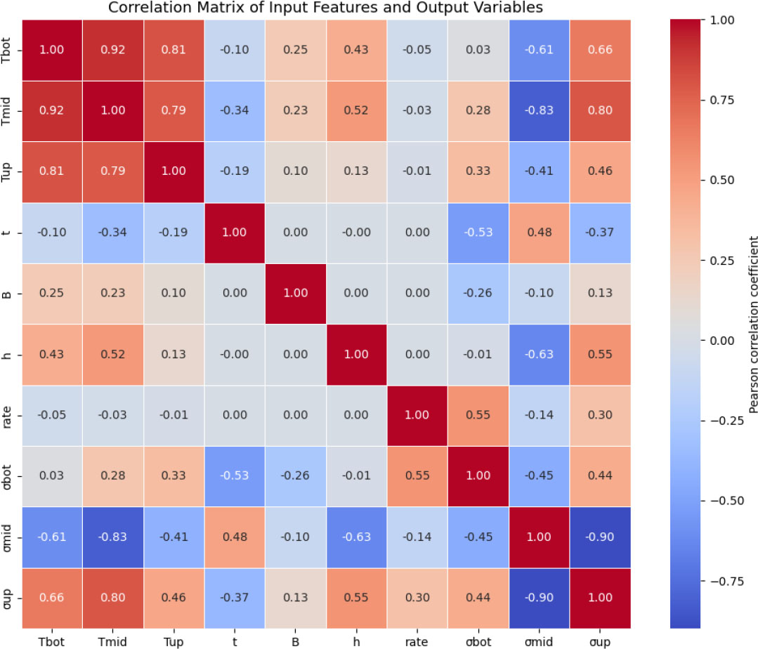
Correlation matrix for all model parameters.
A strong positive correlation is observed between the temperatures at the three key points: ρTbot/Tmid = 0.92, ρTbot/Tup = 0.81, and ρTmidt/Tup = 0.79. This high correlation indicates the coherence of the temperature field across the thickness of the structure. The formation of the stress state in the central part of the structure is influenced by the temperature at the midpoint of the slab thickness ρσ mid/Tmid = -0.83. A similar, but less pronounced, trend is observed for stresses in the lower and upper zones.
The curing time of concrete is moderately related to stresses, both positively and negatively: ρt/σmid = 0.48, ρt/σbot = -0.53, and ρt/σup = -0.37. This parameter reflects the dependence of concrete properties on age, with the concrete strength class having little effect. The hardening rate demonstrates a moderate correlation with stresses in the lower (ρrate/σbot = 0.55) and upper (ρrate/σup = 0.30) zones, confirming the role of hydration kinetics in the development of thermal stresses.
Temperature parameters and slab thickness have the greatest influence on stresses σmid and σup, indicating the key role of the temperature gradient across the thickness of the structure. Curing time has a moderate effect, reflecting the development of the concrete's thermomechanical properties in the early stages. The rate of temperature change and parameters associated with the lower zone of the slab have a secondary, but statistically significant, effect, particularly on σbot and σup. The identified relationships confirm the existence of nonlinear dependencies and the feasibility of using machine learning methods.
Table 6 shows the result of the VIF analysis.
| Sign | VIF |
|---|---|
| Tbot | 11.020124 |
| Tmid | 16.073420 |
| Tup | 4.906047 |
| t | 2.013276 |
| B | 1.211721 |
| h | 2.467970 |
| rate | 1.006731 |
Considering the generally accepted VIF thresholds, it can be concluded that the high values for the temperature features (VIFTbot =11.020124, VIFTmid = 16.073420, VIFTup = 4.906047) are determined by their physical interrelationships and lead to a violation of the assumption of independence of the target variables. Under conditions of pronounced multicollinearity, the linear regression coefficients become unstable, sensitive to noise, and difficult to interpret, and forecast accuracy is significantly reduced.
The CatBoost algorithm was chosen as the primary model. It is robust to multicollinearity, handles highly correlated features correctly, and effectively approximates nonlinear relationships without prior parameter exclusion. This is especially important for analyzing thermal stresses, the formation of which is determined by the complex nonlinear interaction of temperature, geometric, and time factors.
Figure 2 shows the distribution of model residuals for stresses in the lower zone of the slab (σbot) as a function of curing time. The residuals are generally symmetrically distributed around the zero line, indicating the absence of systematic bias in the prediction.
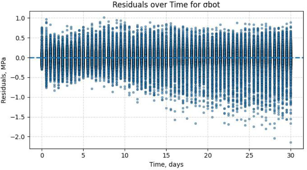
Residuals of the temperature stress forecast σbotover time.
Figure 3 shows the distribution of model residuals for stresses at the center of the slab thickness (σmid) as a function of curing time. The absence of a trend and a uniform distribution of points around zero indicate the random nature of the errors and the adequacy of the model.
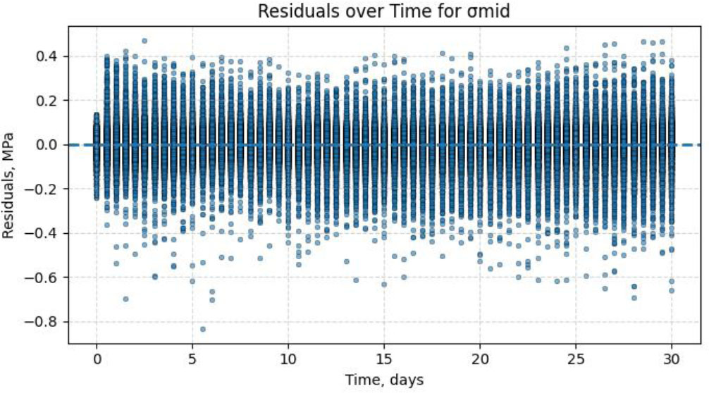
Residuals of the temperature stress σmid forecast over time.
Figure 4 shows the distribution of model residuals for stresses on the top surface of the slab (σup) as a function of curing time. There is no time trend and a uniform distribution of points around zero. In the long term (after 20–30 days), a relative stabilization of the residuals near zero is observed, indicating model convergence or the process reaching a steady state.
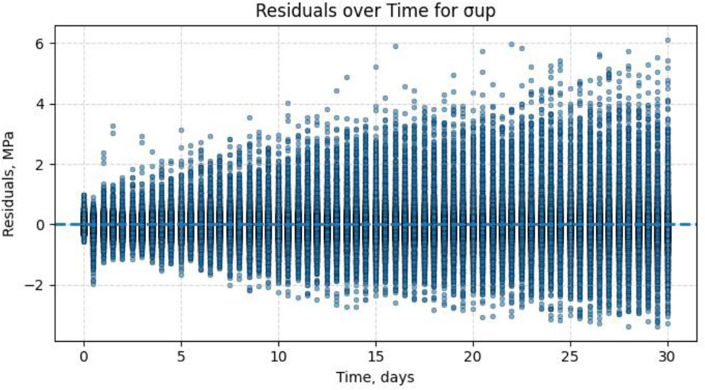
Residuals of the temperature stress σup forecast over time.
The results show that the residuals for all stress components are randomly distributed around zero and do not exhibit a significant time trend. Most residual values are within the range of ±3σ, where σ is the standard deviation, indicating the absence of significant outliers and stable model performance over time.
The forecasting quality indicators are presented in Table 7.
| Variable/Metric | MAE | MSE | RMSE | R2 |
|---|---|---|---|---|
| σbot | 0.130 | 0.035 | 0.180 | 0.996 |
| σmid | 0.383 | 0.384 | 0.619 | 0.995 |
| σup | 0.060 | 0.007 | 0.082 | 0.994 |
The significance of the model parameters ranked by degree of importance for σbot is clearly shown in Fig. (5). The quantitative assessment of the contribution of each parameter is as follows: hardening rate – 99%; time – 96%; concrete class – 47%; slab thickness – 40%; temperature on the upper surface of the slab – 23%; temperature in the middle of the slab thickness – 16%; temperature on the lower surface of the slab – 6%.
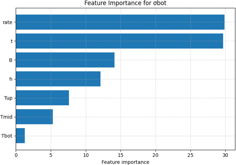
Importance of features for the forecasting σbot values.
The rate of heat release and time have a strong influence on the magnitude of thermal stresses on the bottom surface of the slab. The faster the hydration, the faster the internal temperature rises and the greater the gradient between the bottom (which often rests on a cold foundation or old concrete) and the center. Controlling the rate of strength gain is critical for the bottom surface of the slab.
The significance of the model parameters ranked by degree of importance for σmid is clearly shown in Fig. (6). The quantitative assessment of the contribution of each parameter is as follows: temperature at the middle of the slab thickness – 94%; concrete curing time – 48%; slab thickness – 45%; temperature on the upper surface of the slab – 25%; heat release rate – 23%; concrete class – 10%; stress on the lower surface of the slab – 3%.
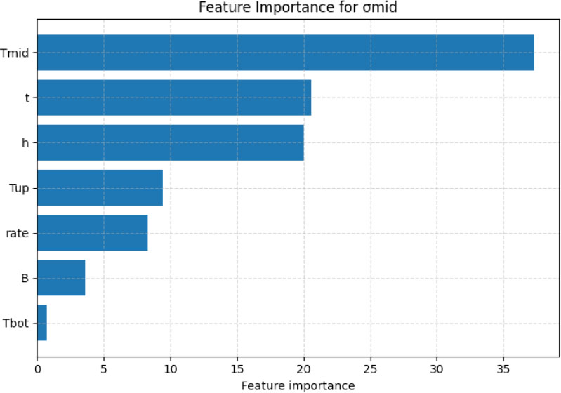
Importance of features for the forecasting σmid values.
For stresses in the middle of the slab thickness, the dominant parameter is the temperature in the middle of the slab thickness, as a direct cause of thermal expansion, as well as the curing time of the concrete and the thickness of the slab.
The significance of the model parameters ranked by degree of importance for σup is clearly shown in Fig. (7). The quantitative assessment of the contribution of each parameter is as follows: temperature at the middle of the slab thickness – 89%; heat release rate – 67%; temperature on the upper surface of the slab – 55%; temperature on the lower surface of the slab – 44%; slab thickness – 33%; curing time – 22%; concrete class – 11%.
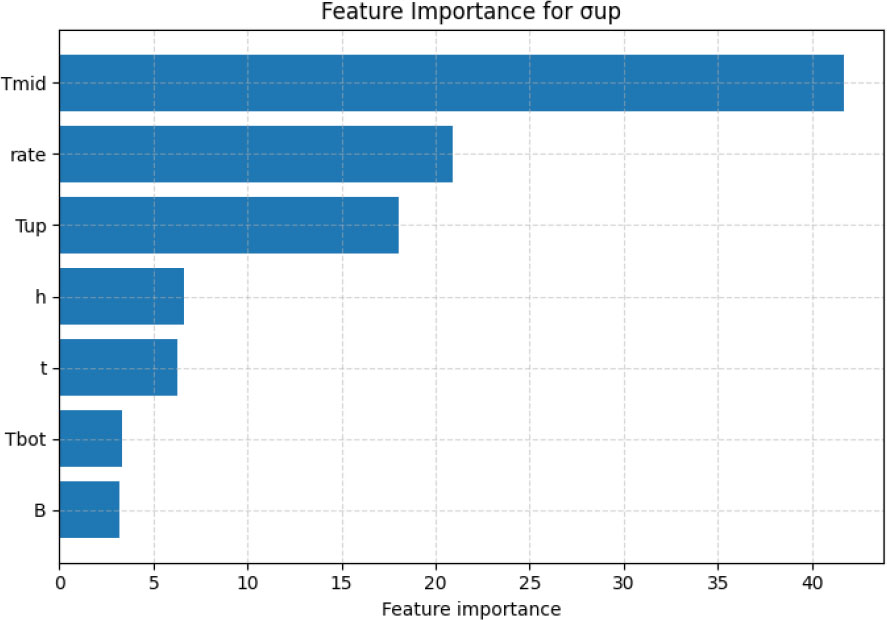
Importance of features for the forecasting σup values.
The stresses on the top surface are largely determined by the temperature regime of the slab's core. The heated core tends to expand, creating a thrust that acts on the cooler surface layers. Thus, the temperature in the core is the primary source of thermal stresses transferred to the top surface.
Multiple cross-validation was performed at different initial values of the random number generator (random seed) for each set of the training subsample to analyze the effect of sample size on the quality of model prediction. The results of the analysis are shown in Fig. (8).
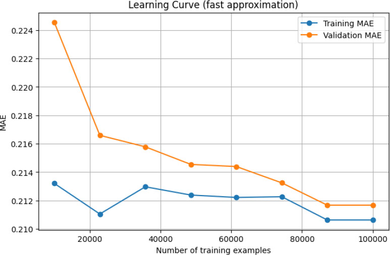
The learning curve of the CatBoost model.
The number of samples in the training dataset correspond the abscissa axis, and the absolute error values in the training and validation subsamples correspond to the ordinate axis. The learning curves of the model are constructed using the Repeated k–Fold Cross–Validation method (Repeated k–Fold CV, k = 5). The orange line is an error in the training sample, and the blue line is an error in the validation sample.
With a small training sample in the range of about 7000 to 2200, there is a significant gap between the average errors in the training and validation subsets, but already in the range of 35000 – 70,000, the difference becomes much smaller. After 70,000, the model stabilizes, and the error is less than 1%. This means that even when using 70-80% of the maximum amount of data, the model demonstrates stable convergence.
The results of repeated training of the model are as follows. For σbot: MAE = 0.10454 ± 0.00032 (MPa); for σmid: MAE = 0.04654 ± 0.00033 (MPa); for σup: MAE = 0.29916 ± 0.00115 (MPa).
During model training, the best parameter values for the CatBoost models were obtained, as presented in Table 8.
| No. | Parameter/Model | σbot | σmid | σup |
|---|---|---|---|---|
| 1 | depth | 6 | 6 | 6 |
| 2 | learning_rate | 0.1 | 0.1 | 0.1 |
| 3 | iterations | 1000 | 1000 | 1000 |
As a result of hyperparameter selection, the grid chose several options as the optimal set: depth {4, 6}; learning_rate {0.05, 0.1}; iterations 1000, while the smallest error was obtained on the set of depth 4, learning_rate 0.1, with a fixed value of the number of iterations of 500. The obtained results confirm not only the quality of the constructed model, but also reveal physically justified dependencies.
4. DISCUSSION
The developed model was also tested on experimental data for a real slab presented in [32]. In that paper, a 2-meter-thick slab was considered. The strength characteristics of the concrete used correspond to class B22.5 according to Russian standards, and the hardening kinetics correspond to rapid-hardening concrete (rate = 1). The experimental values of temperatures at the bottom surface, in the middle of the thickness, and at the top surface are shown in Fig. (9). The temperature at the top surface experienced significant fluctuations due to the variable effects of wind and solar radiation, as well as changing ambient temperatures. Therefore, preliminary smoothing was performed for the parameter before it was fed into the machine learning model.
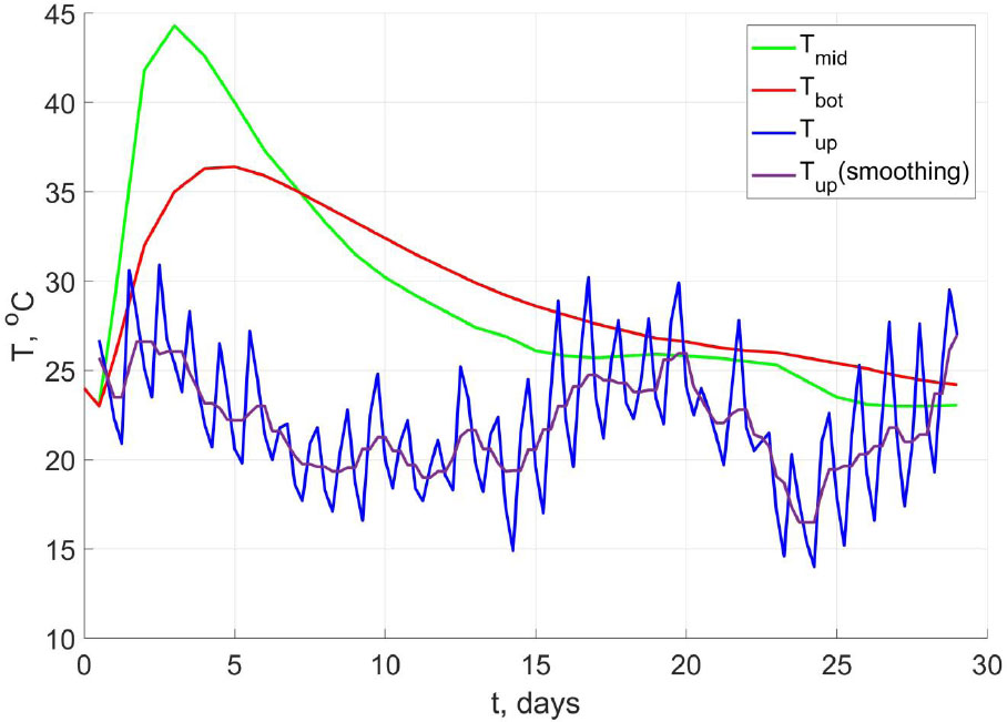
Experimental graphs of temperature changes.
Figure 10 shows a comparison of experimental stress values at the middle of the thickness with the prediction results using the trained model. The trained model demonstrated exceptional prediction accuracy up to 16 days. After this point, cracking was detected in the experiment, accompanied by a drop in stress to near zero. In the time range from 0 to 16 days, the R2 value between the experimental and predicted by CatBoost values is 0.959.
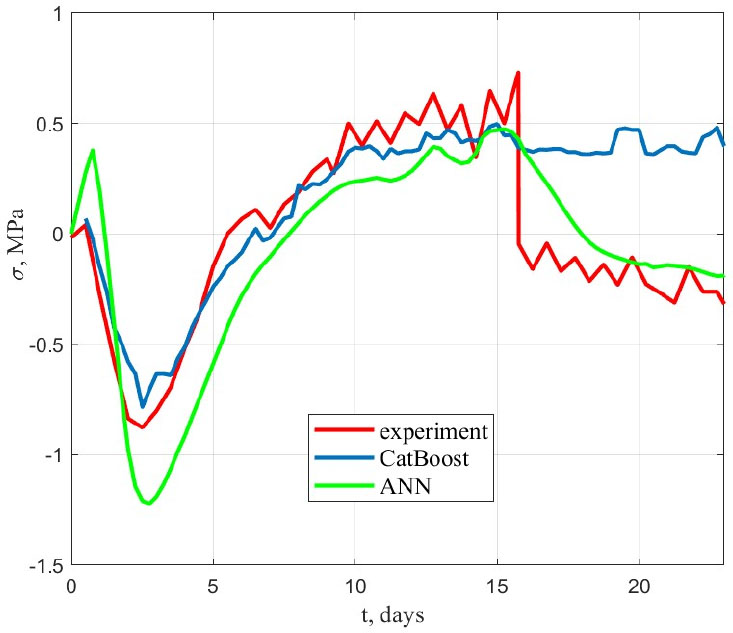
Comparison of experimental results with forecasting results using the CatBoost algorithm and ANN.
Figure 10 also shows the prediction results obtained using the feedforward artificial neural network (ANN) trained on the same dataset. The ANN used had 2 hidden layers of 16 neurons with an activation function in the form of a hyperbolic tangent. The figure shows that the ANN demonstrated lower prediction accuracy compared to CatBoost over the time interval from 0 to 16 days. The difference is particularly noticeable in the compressive stress extremes (-0.877 MPa in the experiment versus -1.22 MPa using ANN). The fact that the artificial neural network shows a drop in stress after 16 days, as in the experiment, is most likely coincidental, since crack formation was not taken into account when forming the training dataset.
5. STUDY LIMITATIONS
The machine learning model was trained on data generated within specific parameter ranges (concrete class B20–B50, slab thickness 0.75–3 m, ambient temperature 5–35 °C, etc.), and its predictive reliability outside these ranges is not guaranteed. The training dataset was obtained from numerical simulations (FEM) rather than experimental measurements; although the FEM model was validated against known results, the ML model inherits any systematic biases or simplifications present in the numerical model. The model predicts stresses in an intact, continuous structure and does not account for stress redistribution or stress drop after crack formation, which limits its applicability once cracking occurs. The approach relies on temperatures measured at only three characteristic points (bottom, middle, top). While sufficient for typical temperature gradients, it may not capture complex three-dimensional thermal fields or localized effects near edges, corners, or embedded cooling pipes.
CONCLUSION
Based on numerical modeling using the finite element method, a representative training dataset of 717,360 records was generated. This dataset was subsequently used to build a machine learning model that predicts stresses at characteristic points of a massive monolithic foundation slab from temperature monitoring data.
Verification of the developed model on independent experimental data confirmed its high predictive ability: the coefficient of determination R2 for stresses at all three control points exceeded 0.99, and the mean absolute error (MAE) was 0.130 MPa for the lower surface, 0.383 MPa for the center, and 0.060 MPa for the upper surface.
The conducted correlation analysis and calculation of variance inflation factors (VIF) revealed significant multicollinearity of the temperature features (VIF up to 16.07). This justifies the inappropriateness of using linear regression models and confirms the correctness of the choice of gradient boosting (CatBoost) as the machine learning algorithm, as it is resistant to highly correlated data and effectively approximates nonlinear dependencies.
An analysis of the feature importance allowed quantification of the contribution of various factors to the formation of the stress state. It was found that the temperature at the center of the slab has the dominant effect on stresses at the middle of the slab (94%), while the heat release rate (99%) and curing time (96%) have the most significant impact on stresses on the lower surface. For the upper surface, the determining factors are the temperature of the central zone (89%) and the heat release rate (67%). Slab thickness and concrete strength class showed a moderate but statistically significant impact on all stress components.
Validation of the model using experimental data demonstrated its exceptional accuracy up to the point of crack formation (16 days). The stress drop recorded after crack formation is not described by the proposed model, which is an objective limitation, as the model is trained to predict stresses in an intact structure without accounting for material discontinuities.
Thus, the proposed approach, which integrates in-situ temperature monitoring data with machine learning methods, eliminates the assumption of a parabolic temperature distribution, which limits the applicability of analytical methods for thick slabs. An additional advantage is the implicit accounting of the evolution of the concrete elastic modulus over time through temperature–time parameters, providing a more realistic description of the stress–strain state in the early stages of hardening. Compared to the finite element method, the developed methodology is orders of magnitude less computationally intensive, enabling its application in engineering practice for rapid (near-real-time) assessment of the risk of early-age cracking directly during construction monitoring.
The proposed method enables prompt decision-making to prevent early cracking when stresses in a structure may reach dangerous levels, such as by using additional surface thermal insulation. Also, based on an assessment of thermal stresses, it is possible to decide whether to strip the structure or stop water cooling once stresses have passed their peak value.
Directions for future research involve expanding the experimental base for temperature stresses during the construction of massive monolithic structures and fine-tuning the model using real measurements as they accumulate.
AUTHOR’S CONTRIBUTIONS
The authors confirm contribution to the paper as follows: A.C.: Conceived and designed the study; V.T.: Developed software; T.K.: Conducted the analysis and drafted the manuscript. All authors reviewed the results and approved the final version of the manuscript.
LIST OF ABBREVIATIONS
| CatBoost | = Categorical Boosting |
| FEM | = Finite Element Method |
| Lasso | = Least Absolute Shrinkage and Selection Operator |
| MAE | = Mean Absolute Error |
| ML | = Machine Learning |
| MSE | = Mean Squared Error |
| RMSE | = Root Mean Square Error |
| VIF | = Variance Inflation Factor |
| XFEM | = eXtended Finite Element Method |
| XGB | = XGBoost |
| ANN | =Artificial Neural Network |
| SHAP | = SHapley Additive exPlanations |
| Repeated k – Fold CV | = Repeated k – Fold Cross – Validation |
AVAILABILITY OF DATA AND MATERIALS
The training dataset is available for download at the link: https://disk.yandex.ru/i/rQLTG-X9AmNvYg.
FUNDING
The study was supported by the grant of the Russian Science Foundation No. 25-19-00164, https://rscf.ru/ project/25-19-00164/.
ACKNOWLEDGEMENTS
The authors would like to acknowledge the administration of Don State Technical University, Russia for their resources and Russian Science Foundation for the financial support.